Gaia Telescope Data Unlocks Hidden Binary Stars at Ultra-Tight Scales
Astronomy

Gaia Telescope Data Unlocks Hidden Binary Stars at Ultra-Tight Scales

A novel data analysis technique bypasses traditional imaging limits to resolve stellar companions down to 0.1 arcseconds using raw telemetry.
By Karan Das
Published:
Email this Article
Gaia Telescope Data Unlocks Hidden Binary Stars at Ultra-Tight Scales
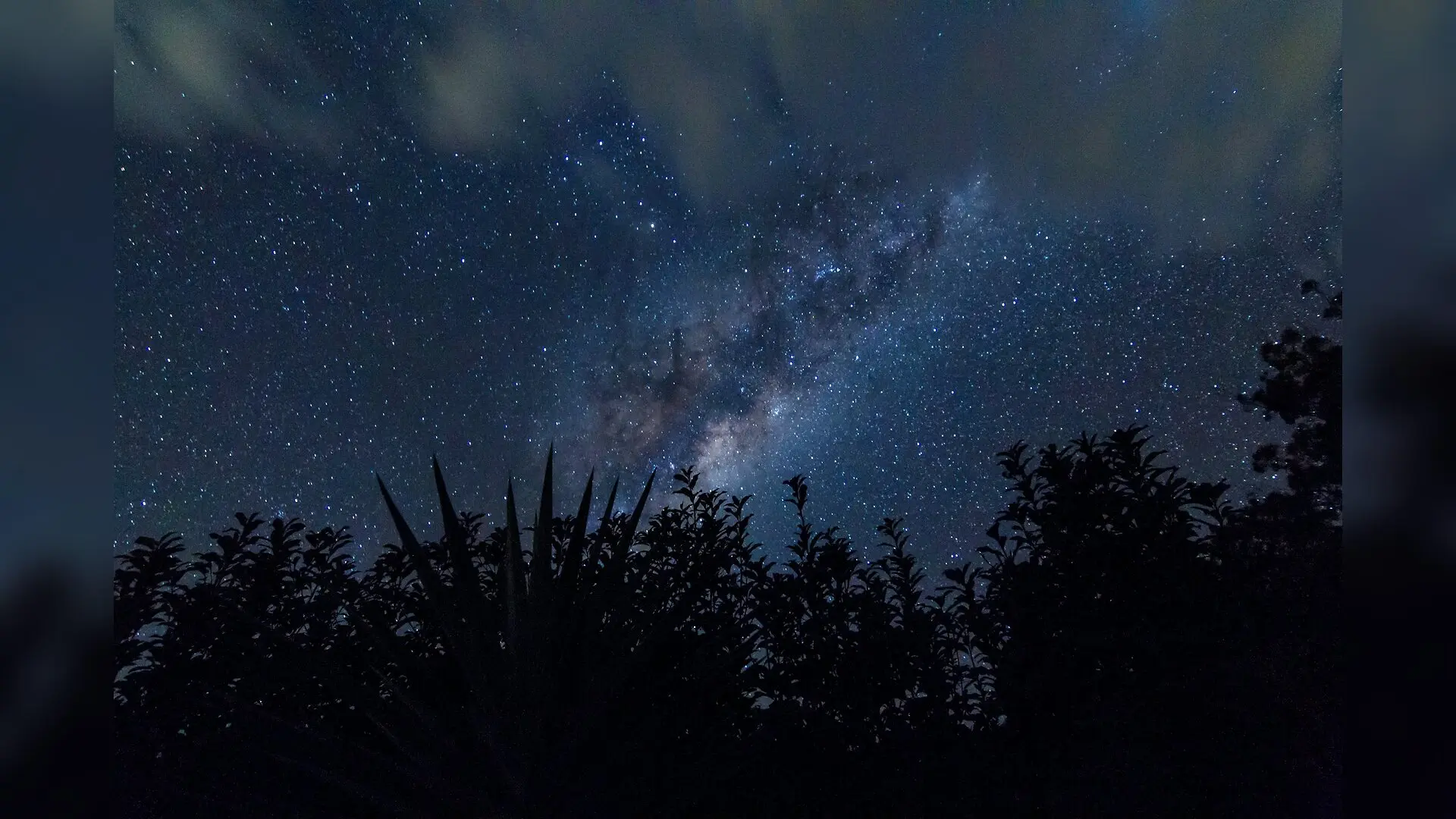
Photo by Photoholgic on Unsplash

A novel data analysis technique reveals that the European Space Agency’s Gaia space telescope can resolve stellar companions separated by just 0.1 arcseconds, far tighter than its standard operational limits. By re-examining the one-dimensional flux profiles transmitted across 50 to 100 observations per sky source, researchers have unlocked a way to map hidden binary systems and measure their orbital motion.

Decoding One-Dimensional Scans for Sub-Pixel Resolution

Gaia records stellar scenes through elongated windows measuring roughly 1 by 2 arcseconds, capturing light at varying scan angles across its multi-year mission. While these scans blend close neighbors into a single overlapping profile, the detailed shape of that light curve changes dynamically as the spacecraft views the system from different directions. The authors of the study, published in the arXiv preprint server, developed a mathematical framework that models these overlapping profiles directly from the raw window data rather than waiting for fully formed two-dimensional images.

To pinpoint individual stars, the team implemented a multi-stage approach beginning with per-window non-negative least squares fitting on a dense grid of point-source profiles. Each individual detection defines a possible line of position on the sky, perpendicular to the instrument scan angle. By accumulating these intersecting lines in what the researchers call a triangulation map, the algorithm identifies candidate companion positions without requiring prior source assignments.
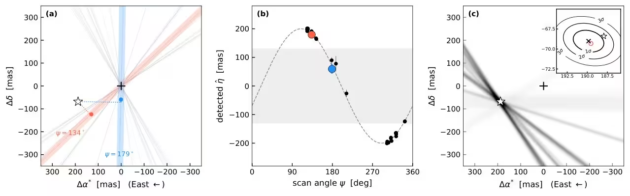
Figure 2: From along-scan detections to a two-dimensional source position. (a) Scan geometry for the simulated pair, with the primary at the origin (cross) and the companion marked by the star. Each line through the origin is the scan axis of one transit, and two transits are highlighted. The dotted segment drops the companion perpendicularly onto the scan axis, and the dot marks the along-scan position measured from the window. Figure 1 shows how a single window is reduced to such along-scan positions. (b) Along-scan detections as a function of scan angle, with formal positional uncertainties. The dashed curve is the injected track, ρ​cos⁡(ψ−φ)\rho\cos(\psi-\varphi). The gray band marks projected separations for which the noise-free blended profile of this pair, with a flux ratio of 0.20.2, has a single peak. This is not a boundary for detecting a second source. (c) The triangulation map combines bands around the sky lines allowed by the detections, with widths set by their positional uncertain
From along-scan detections to a two-dimensional source position. (a) Scan geometry for the simulated pair, with the primary at the origin (cross) and the companion marked by the star. Each line through the origin is the scan axis of one transit, and two transits are highlighted. The dotted segment drops the companion perpendicularly onto the scan axis, and the dot marks the along-scan position measured from the window. Figure 1 shows how a single window is reduced to such along-scan positions. (b) Along-scan detections as a function of scan angle, with formal positional uncertainties. The dashed curve is the injected track, ρ​cos⁡(ψ−φ)\rho\cos(\psi-\varphi). The gray band marks projected separations for which the noise-free blended profile of this pair, with a flux ratio of 0.20.2, has a single peak. This is not a boundary for detecting a second source. (c) The triangulation map combines bands around the sky lines allowed by the detections, with widths set by their positional uncertain Credit: Sahar Shahaf et al. / arXiv

Accounting for Orbital Motion and Contaminants

Many stellar pairs are not static, and their orbital movement over a multi-year campaign can smear traditional detections if left uncorrected. The investigators extended their projection geometry to include relative proper motion, allowing them to trace moving companions and compensate for shifts before performing a joint forward model across all available transits. This dynamical backprojection aligns intersecting sky lines into sharp convergence points.

Testing the pipeline on simulated scenes with multiple stars demonstrated high precision even in crowded fields. For a simulated companion located 75 milliarcseconds away from a primary star with a flux ratio of 0.2, the method achieved a separation precision of roughly 0.1 milliarcseconds and a relative proper-motion precision of about 0.1 milliarcseconds per year. Furthermore, the analysis showed that including neighboring background sources, such as a static star 250 milliarcseconds distant, prevents significant biases in measuring the primary companion.
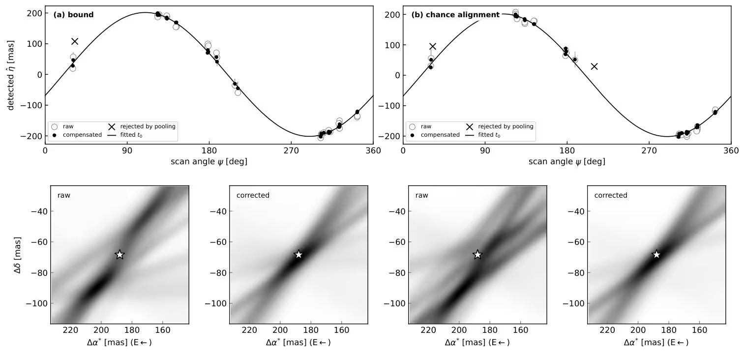
Figure 3: Motion compensation for a bound companion (a) and a chance-aligned background source (b). Both scenes have a separation of 200200 mas at the reference epoch, a flux ratio of 0.30.3, and the uniform noise of Section 4.4, sampled at the same 4747 GOST-predicted transits as Figure 2. Top: along-scan detections before compensation (open circles) and after removing the fitted relative motion and, for the background source, differential parallax (filled points). Crosses mark detections rejected by pooling. The solid curve shows the fitted scene at the reference epoch. The compensation uses the parameters from the joint window fit. Bottom: triangulation maps before and after compensation for each scene. Stars mark the injected position at the reference epoch. Accounting for motion brings the projected detections into closer agreement and concentrates the map near that position.
Motion compensation for a bound companion (a) and a chance-aligned background source (b). Both scenes have a separation of 200200 mas at the reference epoch, a flux ratio of 0.30.3, and the uniform noise of Section 4.4, sampled at the same 4747 GOST-predicted transits as Figure 2. Top: along-scan detections before compensation (open circles) and after removing the fitted relative motion and, for the background source, differential parallax (filled points). Crosses mark detections rejected by pooling. The solid curve shows the fitted scene at the reference epoch. The compensation uses the parameters from the joint window fit. Bottom: triangulation maps before and after compensation for each scene. Stars mark the injected position at the reference epoch. Accounting for motion brings the projected detections into closer agreement and concentrates the map near that position. Credit: Sahar Shahaf et al. / arXiv

Instrumental Limits and Future Applications

The success of this reconstruction relies heavily on an accurate understanding of Gaia’s line-spread function, which describes how the telescope optics spread out point sources. Small errors in the effective wavenumber, which dictates the profile width based on stellar color, can introduce systematic shifts in fitted positions and occasionally mimic false companions. The authors quantified these color-induced biases and noted that future data releases will require careful calibration of instrumental profiles to maintain high astrometric fidelity.

Despite these challenges, the capability to extract 0.1-arcsecond astrometry from one-dimensional telemetry expands Gaia’s scientific reach. By combining these windows with external measurements and forward modeling, astronomers can uncover faint stellar companions, measure short orbital arcs, and investigate dynamical systems that would otherwise remain unresolved in standard wide-field surveys.

The study was posted to the arXiv preprint server on November 16, 2026.

Fact Checked

This article has been fact checked for accuracy, with information verified against reputable sources. Learn more about us and our editorial process.

Last reviewed on .

Article history

  • Latest version

Reference(s)

  1. Shahaf, Sahar. “Gaia as a 0.1 arcsec point-source survey across the sky: dynamical scene reconstruction from one-dimensional scans.” arXiv.org <http://arxiv.org/abs/2611.21510v1>.

Cite this page:

Das, Karan. “Gaia Telescope Data Unlocks Hidden Binary Stars at Ultra-Tight Scales.” BioScience. BioScience ISSN 2521-5760, 17 November 2026. <https://www.bioscience.com.pk/en/subject/astronomy/gaia-as-a-0-1-arcsec-point-source-survey-across-the-sky-dynamical-scene-reconstruction-from-one-dimensional-scans>. Das, K. (2026, November 17). “Gaia Telescope Data Unlocks Hidden Binary Stars at Ultra-Tight Scales.” BioScience. ISSN 2521-5760. Retrieved November 17, 2026 from https://www.bioscience.com.pk/en/subject/astronomy/gaia-as-a-0-1-arcsec-point-source-survey-across-the-sky-dynamical-scene-reconstruction-from-one-dimensional-scans Das, Karan. “Gaia Telescope Data Unlocks Hidden Binary Stars at Ultra-Tight Scales.” BioScience. ISSN 2521-5760. https://www.bioscience.com.pk/en/subject/astronomy/gaia-as-a-0-1-arcsec-point-source-survey-across-the-sky-dynamical-scene-reconstruction-from-one-dimensional-scans (accessed November 17, 2026).
  • Posted by
End of the article