Modified Gravity Models Struggle to Match Standard Cosmology in New Study
Physics

Modified Gravity Models Struggle to Match Standard Cosmology in New Study

Anisotropic universe models in modified gravity can mimic cosmic acceleration, but statistical comparisons favor the standard cosmological framework.
By Farah Siddiqui
Published:
Email this Article
Modified Gravity Models Struggle to Match Standard Cosmology in New Study
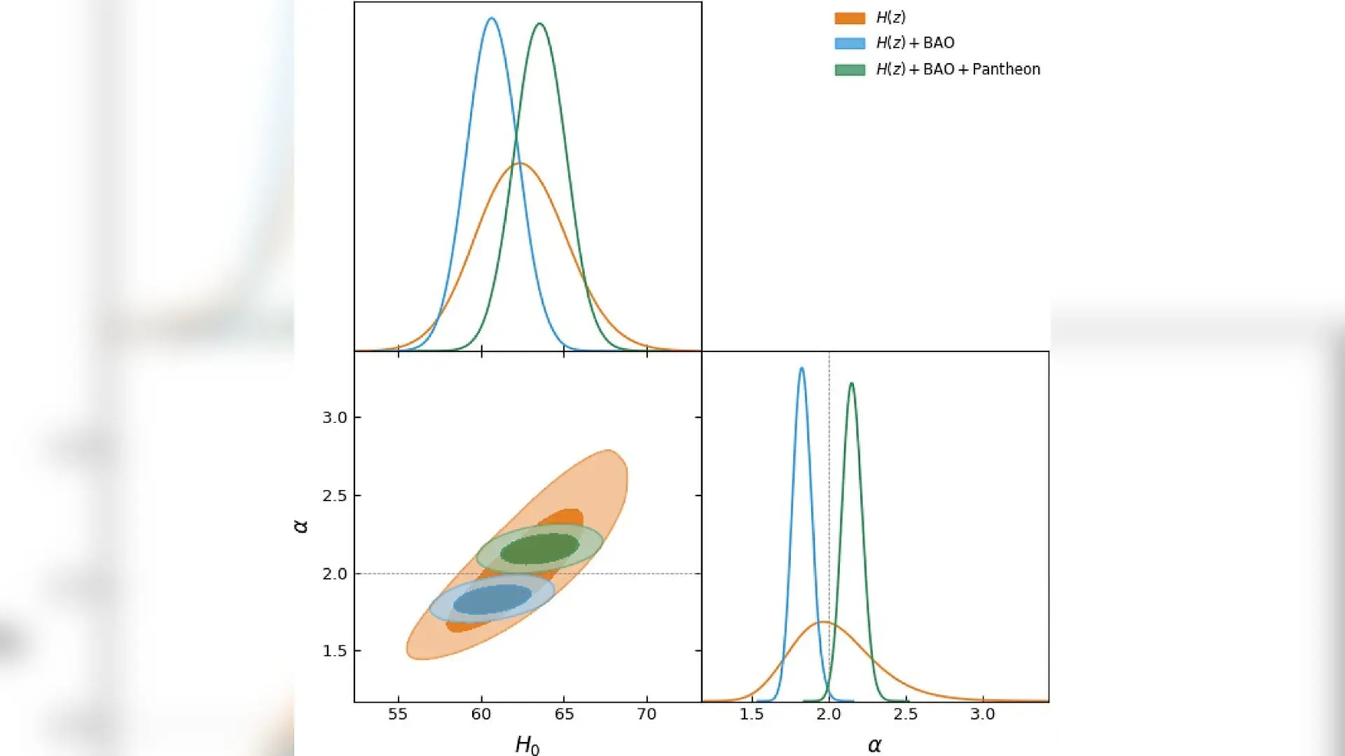
Comparison of the marginalized Model I constraints in the H0\documentclass[12pt]{minimal} \usepackage{amsmath} \usepackage{wasysym} \usepackage{amsfonts} \usepackage{amssymb} \usepackage{amsbsy} \usepackage{mathrsfs} \usepackage{upgreek} \setlength{\oddsidemargin}{-69pt} \begin{document}$$H_0$$\end{document}–α\documentclass[12pt]{minimal} \usepackage{amsmath} \usepackage{wasysym} \usepackage{amsfonts} \usepackage{amssymb} \usepackage{amsbsy} \usepackage{mathrsfs} \usepackage{upgreek} \setlength{\oddsidemargin}{-69pt} \begin{document}$$\alpha$$\end{document} plane obtained from H(z), H(z)+BAO\documentclass[12pt]{minimal} \usepackage{amsmath} \usepackage{wasysym} \usepackage{amsfonts} \usepackage{amssymb} \usepackage{amsbsy} \usepackage{mathrsfs} \usepackage{upgreek} \setlength{\oddsidemargin}{-69pt} \begin{document}$$H(z)+\textrm{BAO}$$\end{document}, and H(z)+BAO+Pantheon\documentclass[12pt]{minimal} \usepackage{amsmath} \usepackage{wasysym} \usepackage{amsfonts} \usepackage{amssymb} \ Joshi et al. / The European Physical Journal Plus

Cosmological models assuming a perfectly uniform Universe struggle to capture potential wrinkles in the fabric of space, prompting physicists to test alternative geometric theories. A new study examining anisotropic models in modified gravity suggests that while these equations can generate accelerated expansion, they currently fail to outmatch the standard cosmological model when tested against comprehensive datasets.

The standard model of cosmology, known as the ΛCDM framework, successfully describes a flat and isotropic universe governed by cold dark matter and a cosmological constant. However, anomalies on large angular scales observed in the cosmic microwave background point toward a potential mild anisotropy in the geometry of the Universe. To address these geometric hints, researchers frequently turn to locally rotationally symmetric Bianchi Type-I spacetimes. These models allow for distinct expansion rates along different spatial directions, departing from traditional isotropic assumptions.

To explore how such an anisotropic universe evolves, a team of researchers investigated alternative gravitational dynamics via f(R) gravity, a theoretical approach that replaces the standard Ricci scalar curvature in the Einstein-Hilbert action with a more general function of R. By introducing nonlinear curvature terms, the theory can generate an effective dark energy behavior without requiring exotic matter fields. The study, published in The European Physical Journal Plus, constructs two distinct classes of vacuum anisotropic models and tests their mean-background expansion histories against modern observational data.
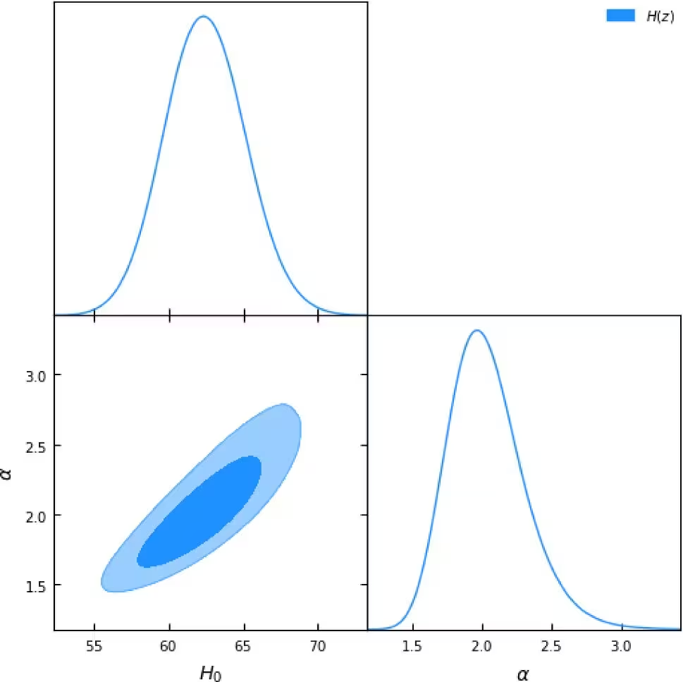
Fig. 1: Marginalized posterior distributions for the Model I parameters H0\documentclass[12pt]{minimal} \usepackage{amsmath} \usepackage{wasysym} \usepackage{amsfonts} \usepackage{amssymb} \usepackage{amsbsy} \usepackage{mathrsfs} \usepackage{upgreek} \setlength{\oddsidemargin}{-69pt} \begin{document}$$H_0$$\end{document} and α\documentclass[12pt]{minimal} \usepackage{amsmath} \usepackage{wasysym} \usepackage{amsfonts} \usepackage{amssymb} \usepackage{amsbsy} \usepackage{mathrsfs} \usepackage{upgreek} \setlength{\oddsidemargin}{-69pt} \begin{document}$$\alpha$$\end{document} obtained from the H(z) data alone. The one- and two-dimensional distributions show the corresponding 68% and 95% credible regions
Marginalized posterior distributions for the Model I parameters H0\documentclass[12pt]{minimal} \usepackage{amsmath} \usepackage{wasysym} \usepackage{amsfonts} \usepackage{amssymb} \usepackage{amsbsy} \usepackage{mathrsfs} \usepackage{upgreek} \setlength{\oddsidemargin}{-69pt} \begin{document}$$H_0$$\end{document} and α\documentclass[12pt]{minimal} \usepackage{amsmath} \usepackage{wasysym} \usepackage{amsfonts} \usepackage{amssymb} \usepackage{amsbsy} \usepackage{mathrsfs} \usepackage{upgreek} \setlength{\oddsidemargin}{-69pt} \begin{document}$$\alpha$$\end{document} obtained from the H(z) data alone. The one- and two-dimensional distributions show the corresponding 68% and 95% credible regions Credit: Joshi et al. / The European Physical Journal Plus

How Do Anisotropic Gravity Models Function?

The researchers derived the gravitational field equations for an anisotropic universe by assuming a proportional relationship between the expansion scalar and the shear scalar. This approach simplifies the dynamics through a constant parameter, denoted as k, which characterizes the level of directional anisotropy. When k equals one, the universe recovers complete spatial isotropy.

Within this modified framework, the team reconstructed two specific classes of cosmological models. The first assumes a power-law dependence of the derivative of f(R) with respect to the mean Hubble parameter, while the second links the logarithmic time evolution of f(R) directly to the expansion rate. Both formulations result in a constant deceleration parameter, meaning that the expansion rate neither speeds up nor slows down dynamically over cosmic time within a single model run.

What Did the Observational Data Reveal?

The team employed a Bayesian Markov chain Monte Carlo statistical analysis to test the free parameters of the reconstructed models against three primary datasets. These included 30 cosmic chronometer Hubble parameter measurements covering redshifts up to $z = 1.96$, 17 baryon acoustic oscillation data points, and the Pantheon Type Ia supernova sample consisting of 1,048 confirmed stellar explosions.
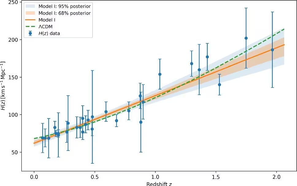
Fig. 2: Observed H(z) data with the posterior-mean reconstruction of Model I. The dashed curve corresponds to the best-fit Λ\documentclass[12pt]{minimal} \usepackage{amsmath} \usepackage{wasysym} \usepackage{amsfonts} \usepackage{amssymb} \usepackage{amsbsy} \usepackage{mathrsfs} \usepackage{upgreek} \setlength{\oddsidemargin}{-69pt} \begin{document}$$\Lambda$$\end{document}CDM cosmology
Observed H(z) data with the posterior-mean reconstruction of Model I. The dashed curve corresponds to the best-fit Λ\documentclass[12pt]{minimal} \usepackage{amsmath} \usepackage{wasysym} \usepackage{amsfonts} \usepackage{amssymb} \usepackage{amsbsy} \usepackage{mathrsfs} \usepackage{upgreek} \setlength{\oddsidemargin}{-69pt} \begin{document}$$\Lambda$$\end{document}CDM cosmology Credit: Joshi et al. / The European Physical Journal Plus

The statistical outcomes varied depending on the dataset combination used. When evaluated against cosmic chronometer data alone, the models hovered near a coasting universe state where the deceleration parameter is close to zero. The inclusion of baryon acoustic oscillation data shifted the preferred parameter space toward a mild deceleration branch. Conversely, adding the Pantheon supernova sample pushed the joint data fit onto an accelerating branch with a deceleration parameter of approximately $q \simeq -0.05$.

Why Does the Standard Model Still Prevail?

Despite the ability of the reconstructed models to accommodate an accelerating phase when using the full combined dataset, statistical comparison tests reveal clear limitations. The researchers utilized the Akaike information criterion and Bayesian information criterion to compare their modified gravity solutions against the standard flat ΛCDM model. For the complete dataset combination, the differences in these information criteria reached approximately $102.6$, indicating a strong statistical preference for the standard model.
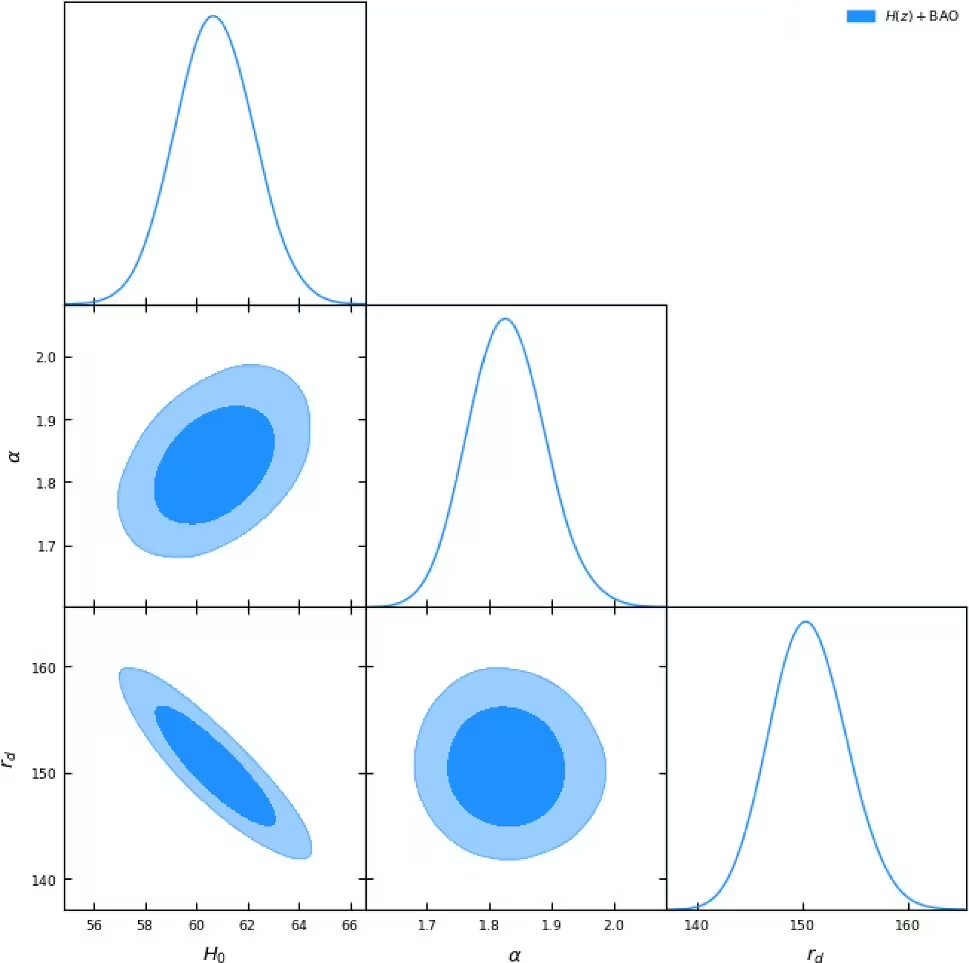
Fig. 3: Marginalized posterior distributions for the Model I parameters H0\documentclass[12pt]{minimal} \usepackage{amsmath} \usepackage{wasysym} \usepackage{amsfonts} \usepackage{amssymb} \usepackage{amsbsy} \usepackage{mathrsfs} \usepackage{upgreek} \setlength{\oddsidemargin}{-69pt} \begin{document}$$H_0$$\end{document}, α\documentclass[12pt]{minimal} \usepackage{amsmath} \usepackage{wasysym} \usepackage{amsfonts} \usepackage{amssymb} \usepackage{amsbsy} \usepackage{mathrsfs} \usepackage{upgreek} \setlength{\oddsidemargin}{-69pt} \begin{document}$$\alpha$$\end{document}, and rd\documentclass[12pt]{minimal} \usepackage{amsmath} \usepackage{wasysym} \usepackage{amsfonts} \usepackage{amssymb} \usepackage{amsbsy} \usepackage{mathrsfs} \usepackage{upgreek} \setlength{\oddsidemargin}{-69pt} \begin{document}$$r_d$$\end{document} obtained from the combined H(z)+BAO\documentclass[12pt]{minimal} \usepackage{amsmath} \usepackage{wasysym} \usepackage{amsfonts} \usepackage{amssymb} \usepackage{amsbsy} \u
Marginalized posterior distributions for the Model I parameters H0\documentclass[12pt]{minimal} \usepackage{amsmath} \usepackage{wasysym} \usepackage{amsfonts} \usepackage{amssymb} \usepackage{amsbsy} \usepackage{mathrsfs} \usepackage{upgreek} \setlength{\oddsidemargin}{-69pt} \begin{document}$$H_0$$\end{document}, α\documentclass[12pt]{minimal} \usepackage{amsmath} \usepackage{wasysym} \usepackage{amsfonts} \usepackage{amssymb} \usepackage{amsbsy} \usepackage{mathrsfs} \usepackage{upgreek} \setlength{\oddsidemargin}{-69pt} \begin{document}$$\alpha$$\end{document}, and rd\documentclass[12pt]{minimal} \usepackage{amsmath} \usepackage{wasysym} \usepackage{amsfonts} \usepackage{amssymb} \usepackage{amsbsy} \usepackage{mathrsfs} \usepackage{upgreek} \setlength{\oddsidemargin}{-69pt} \begin{document}$$r_d$$\end{document} obtained from the combined H(z)+BAO\documentclass[12pt]{minimal} \usepackage{amsmath} \usepackage{wasysym} \usepackage{amsfonts} \usepackage{amssymb} \usepackage{amsbsy} \u Credit: Joshi et al. / The European Physical Journal Plus

Furthermore, the study highlighted notable theoretical constraints. Because the deceleration parameter remains strictly constant in both reconstructed models, neither configuration can describe the physical transition from an early matter-dominated decelerating epoch to the current accelerated expansion phase. Additionally, the specific functional forms encounter theoretical hurdles regarding energy conditions and stability criteria on certain curvature branches.

The authors note that future investigations could overcome these limitations by adopting more flexible reconstruction schemes that allow for a time-dependent deceleration parameter. Incorporating directional photon propagation and individual sky coordinates for observational sources would also enable researchers to constrain spatial anisotropy directly, providing a sharper test for modified gravity theories.

The research was published in The European Physical Journal Plus on November 6, 2026.

Fact Checked

This article has been fact checked for accuracy, with information verified against reputable sources. Learn more about us and our editorial process.

Last reviewed on .

Article history

  • Latest version

Reference(s)

  1. Joshi, Shraddha., et al. “Constraining anisotropic f(R) cosmologies through observational data analysis.” The European Physical Journal Plus, vol. 141, no. 11, November 6, 2026 Springer Science and Business Media LLC, doi: 10.1140/epjp/s13360-026-08512-9. <https://doi.org/10.1140/epjp/s13360-026-08512-9>.

Cite this page:

Siddiqui, Farah. “Modified Gravity Models Struggle to Match Standard Cosmology in New Study.” BioScience. BioScience ISSN 2521-5760, 06 November 2026. <https://www.bioscience.com.pk/en/subject/physics/constraining-anisotropic-f-r-cosmologies-through-observational-data-analysis>. Siddiqui, F. (2026, November 06). “Modified Gravity Models Struggle to Match Standard Cosmology in New Study.” BioScience. ISSN 2521-5760. Retrieved November 06, 2026 from https://www.bioscience.com.pk/en/subject/physics/constraining-anisotropic-f-r-cosmologies-through-observational-data-analysis Siddiqui, Farah. “Modified Gravity Models Struggle to Match Standard Cosmology in New Study.” BioScience. ISSN 2521-5760. https://www.bioscience.com.pk/en/subject/physics/constraining-anisotropic-f-r-cosmologies-through-observational-data-analysis (accessed November 06, 2026).
End of the article